CORRELATION ANALYSIS

While studying two variables at the same time, if it is found that the change in one variable is reciprocated by a corresponding change in the other variable either directly or inversely, then the two variables are known to be associated or correlated.

Otherwise, the two variables are known to be dissociated or uncorrelated or independent. There are two types of correlation.

(i) Positive correlation

(ii) Negative correlation

Positive Correlation

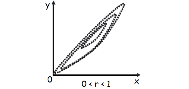
If two variables move in the same direction i.e. an increase (or decrease) on the part of one variable introduces an increase (or decrease) on the part of the other variable, then the two variables are known to be positively correlated.

As for example, height and weight, yield and rainfall, profit and investment etc. are positively correlated.

Negative Correlation

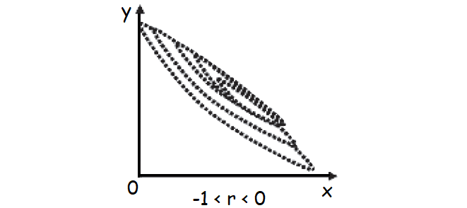
On the other hand, if the two variables move in the opposite directions i.e. an increase (or a decrease) on the part of one variable results a decrease (or an increase) on the part of the other variable, then the two variables are known to have a negative correlation.

For example, the price and demand of an item, the profits of Insurance Company and the number of claims it has to meet etc. are examples of variables having a negative correlation.

The two variables are known to be uncorrelated if the movement on the part of one variable does not produce any movement of the other variable in a particular direction.

As for example, shoe-size and intelligence are uncorrelated.

Measures of Correlation

We consider the following measures of correlation :

(a) Scatter diagram

(b) Karl Pearson’s Product moment correlation coefficient

(c) Spearman’s rank correlation co-efficient

(d) Co-efficient of concurrent deviations

Correlation Analysis - Review

It is obvious that we take recourse to correlation analysis when we are keen to know whether two variables under study are associated or correlated and if correlated, what is the strength of correlation.

The best measure of correlation is provided by Pearson’s correlation coefficient.

However, one severe limitation of this correlation coefficient, as we have already discussed, is that it is applicable only in case of a linear relationship between the two variables.

If two variables x and y are independent or uncorrelated then obviously the correlation coefficient between x and y is zero.

However, the converse of this statement is not necessarily true i.e. if the correlation coefficient, due to Pearson, between two variables comes out to be zero, then we cannot conclude that the two variables are independent.

All that we can conclude is that no linear relationship exists between the two variables. This, however, does not rule out the existence of some non linear relationship between the two variables.

For example, if we consider the following pairs of values on two variables x and y.

(–2, 4), (–1, 1), (0, 0), (1, 1) and (2, 4),

then

cov (x, y) = (–2 + 4) + (–1 + 1) + (0 x 0) + (1 x 1) + (2 x 4)

= 0

as arithmetic mean of x = 0.

Thus,

r = 0

This does not mean that x and y are independent. In fact the relationship between x and y is y = x².

Thus it is always wiser to draw a scatter diagram before reaching conclusion about the existence of correlation between a pair of variables.

There are some cases when we may find a correlation between two variables although the two variables are not causally related.

This is due to the existence of a third variable which is related to both the variables under consideration.

Such a correlation is known as spurious correlation or non-sense correlation.

As an example, there could be a positive correlation between production of rice and that of iron in India for the last twenty years due to the effect of a third variable time on both these variables.

It is necessary to eliminate the influence of the third variable before computing correlation between the two original variables.

Coefficient of Determination

Correlation coefficient measuring a linear relationship between the two variables indicates the amount of variation of one variable accounted for by the other variable.

A better measure for this purpose is provided by the square of the correlation coefficient, Known as ‘coefficient of determination’. This can be interpreted as the ratio between the explained variance to total variance i.e.

Thus a value of 0.6 for r indicates that (0.6)² x 100% or 36 per cent of the variation has been accounted for by the factor under consideration and the remaining 64 per cent variation is due to other factors.

Coefficient of Non-Determination

The ‘coefficient of non-determination’ is given by (1 – r²) and can be interpreted as the ratio of unexplained variance to the total variance.

Therefore,

coefficient of non-determination = (1 – r²)

Kindly mail your feedback to v4formath@gmail.com

We always appreciate your feedback.