MATH DICTIONARY J

Jacobian : 

Assume that the variables x, y, z are expressed with the help of other three variables u, v, w and the change of variable functions

x = x(u, v, w), y = y(u, v, w), z = z(u, v, w)

are continuously differentiable. Then the matrix

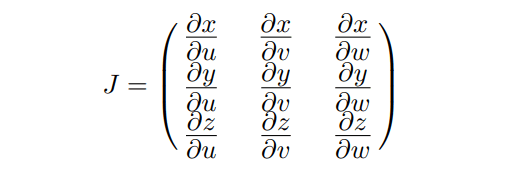
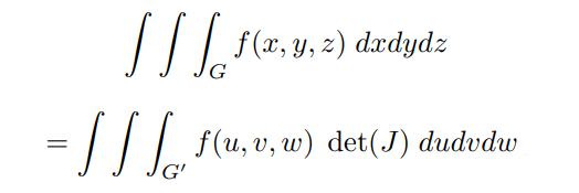
is called the Jacobian matrix of the transformation. The importance of this matrix is that the determinant of J plays important role in calculating integrals by change of variable. The following theorem holds:

Let the function f(x, y, z) be defined and integrable in some region G and let the change of variable formulas

x = x(u, v, w), y = y(u, v, w), z = z(u, v, w)

transform G to some other region G0 . Then

Joint Variation :

The name of many possible relations between three or more variables. The most common are :

1. z varies directly with x and y means that there is a real number k ≠ 0, such that

z = kxy

2. z varies directly with x and inversely with y means 

z = k(x/y) 

3. z varies directly with x 2 and inversely with y means

z = kx²y

There are many other possibilities including more variables. See also inverse variation and direct variation.

Jordan Curve :

Let I = [a, b] be an interval and the functions

x = f(t) and y = g(t)

are defined on that interval. These equations define a plane parametric curve. This curve is called Jordan curve if

1. The functions f, g are continuous

2. The curve is closed, meaning that

f(a) = f(b), g(a) = g(b)

3. The curve is simple, i.e. f(t₁) ≠ f(t₂) except the endpoints, and similarly g(t₁) ≠ g(t₂). Jordan curves in the space are defined in the same way.

Jordan Decomposition :

The Jordan matrix decomposition is the decomposition of a square matrix  M into the form

M = SJS^-1

where  M and  J are similar matrices, J is a matrix of Jordan canonical form and S^-1 is the matrix inverse of S.  In other words, M is a similarity transformation of a matrix J in Jordan canonical form.

Jordan Domain :

A plane region that is bounded by a Jordan curve.

Jordan Form of Matrix :

A block-diagonal square matrix, that could be written in the form.

where each J_k is itself a square matrix. The diagonal elements of this block-matrix are all the same, the sub-diagonal consists of all 1’s, and all the other elements of the matrix are zeros :

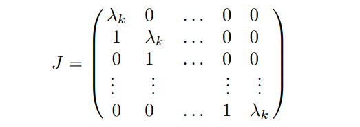
The entries on diagonal are the eigenvalues of the matrix. These type of matrices are called simple Jordan matrix. Every square matrix is similar to a matrix of the Jordan form.

Jump :

The absolute value of the difference between the left-hand and right-hand limits of a given function, i.e.

|(f(x₊) – f(x_-)|

Jump Discontinuity :

A function f(x) is said to have jump discontinuity at some point x = c, if both left-hand and right-hand limits of the function at that point exist, but are not equal :

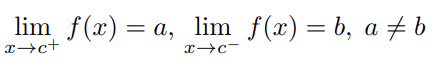
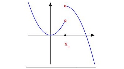
The Heaviside function is an example of a function with jump discontinuity at point 0.

Joint Probability :

The probability of event A and event B happening at the same time.

Joint Probability Function :

A function that gives the probability that each of two or more random variables takes at a particular value.

Joint Cumulative Distribution Function :

For two random variables X and Y, the joint cumulative distribution function is the function F defined by

F(x, y) = P(X ≤ x, Y ≤ y)

The term applies also to the generalization of this to more than two random variables. For two variables, it may be called the bivariate and, for more than two, the multivariate cumulative distribution function.

Joint Distribution :

The joint distribution of two or more random variables is concerned with the way in which the probability of their taking certain values, or values within certain intervals, varies.

It may be given by the joint cumulative distribution function. More commonly, the joint distribution of some number of discrete random variables is given by their joint probability mass function, and that of some number of continuous random variables by their *joint probability density function.

For two variables it may be called the bivariate and, for more than two, the multivariate distribution.

Joint Probability Density Function :

For two continuous random variables X and Y, the joint probability density function is the function f such that

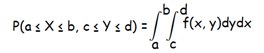
The term applies also to the generalization of this to more than two random variables. For two variables, it may be called the bivariate and, for more than two, the multivariate probability density function.

Joint Probability Mass Function :

For two discrete *random variables X and Y, the joint probability mass function is the function p such that

p(x_i, y_j) = P(X = x_i, Y = y_j),

for all i and j. The term applies also to the generalization of this to more than two random variables. For two variables, it may be called the bivariate and, for more than two, the multivariate probability mass function.

Kindly mail your feedback to v4formath@gmail.com

We always appreciate your feedback.